PyMC3’s “trace” object and “traceplot” function are pretty handy to examine the posterior distributions.
Q1: What’s the suggested way to do in Edward?
I couldn’t find a reference, so below is what I do currently:
# Use a simple linear regression as an example:
import pandas as pd
import numpy as np
import tensorflow as tf
import edward as ed

def generateData(intercept=1, slope=3, noise=1, n_points=20):
    df = pd.DataFrame({'x': np.random.uniform(-3, 3, size=n_points)})
    df['y'] = intercept + slope * df['x'] + np.random.np.random.normal(0, scale=noise, size=n_points)
    df = df.sort_values(['x'], ascending=True).reset_index(drop=True)
    return df

intercept = 1; slope = 3; noise = 1
np.random.seed(99)
data = generateData(intercept=intercept, slope=slope, noise=noise)  #, n_points=n_points)

#
N = 20
D = 1
X = tf.placeholder(tf.float32, [N, D])
sigma = ed.models.Chi2(df=3.0)
w = ed.models.Normal(loc=tf.zeros(D), scale=tf.ones(D)*10.0)
b = ed.models.Normal(loc=tf.zeros(1), scale=tf.ones(1)*10.0)
y = ed.models.Normal(loc=ed.dot(X, w)+b, scale=tf.ones(N)*sigma)

T = 10000

qs = ed.models.Empirical(params=tf.Variable(tf.ones(T)))
qw = ed.models.Empirical(params=tf.Variable(tf.random_normal((T, D) )))
qb = ed.models.Empirical(params=tf.Variable(tf.random_normal((T, 1) )))

inference = ed.HMC({sigma: qs, w: qw, b: qb},
                   data={X: data[['x']].values, y: data['y'].values})
inference.run(step_size=3e-3)

# After the inference process is finished, generate posterior samples
n_samples = 1000
w_posterior = qw.sample(n_samples).eval().ravel()
b_posterior = qb.sample(n_samples).eval().ravel()
s_posterior = qs.sample(n_samples).eval().ravel()
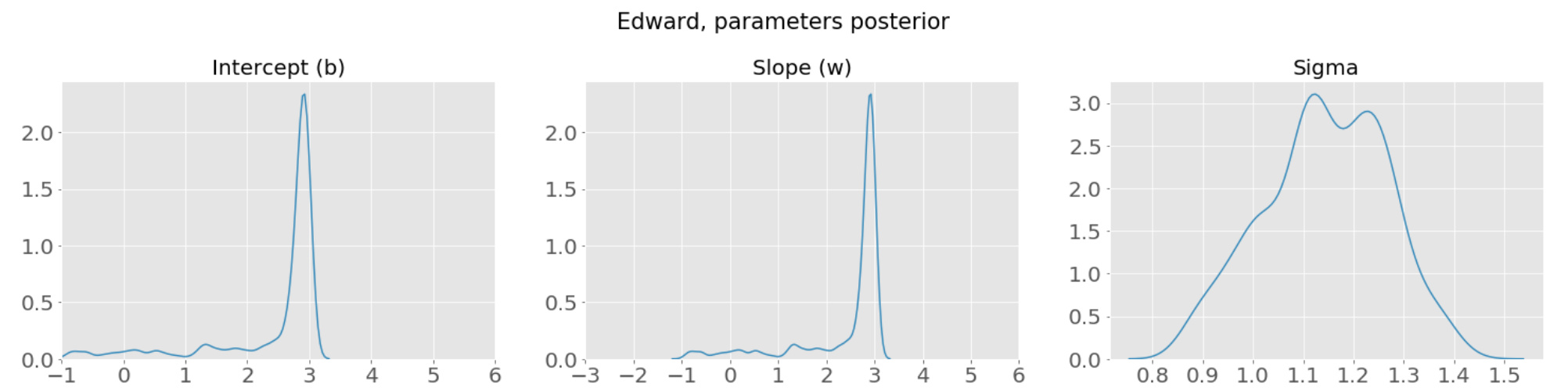
The posterior distributions of the above three parameters are as follow:
Q2: Is there a way to get the posterior samples from the “inference” object? It seems a bit awkward that I specified “T=10000” for the MCMC runs but I wasn’t able to use the samples there, and had to generate extra “n_samples = 1000” samples to examine the posteriors.
I’m new to Edward, so any suggestions are welcome and appreciated!